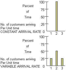
There are many levels or degrees of complexity that can exist within queues. We will start with the simplest situation:

• Customers arrive at a constant rate.
• There is a single server.
• The server processes customers at a constant rate.

Consider a metal-craft factory and a machine that is used to "smooth" the raw items (beer mugs and ashtrays). These items are then taken by belt to another machine which sprays a lacquer finish on each item. One could regard the smooth items as customers for the spray machine and the spray machine as a service facility. In this case customers arrived at a constant rate with approximately 12 second between arrivals. The time required to spray (service) an item was approximately 7 seconds.
1. For these arrival and processing rates (of 1 arrival every 12 seconds and 1 item processed every 7 second) and assuming no breakdowns, what percent of the time is the sprayer actually working.?

2. How many items are in the queue to the sprayer after 5 minutes of operation, if the items which arrived exactly 5 minutes after the operation started is ignored?

3. What is the fastest arrival rate of items to the spraying machine which will not allow for any queue to build up?

4. At the fastest arrival rate, what percent of the time is the sprayer actually working?

5. Suppose one item arrives for processing every x seconds and processing each item required y seconds. What happens to the queue if the following order relations hold between x and y?
   • x < y
   • x = y
   • x > y

6. If x < y for a certain processor in a production system, name 2 ways to overcome the problem.

   One way which may have come to mind is the addition of a second server or sprayer. In fact, it is through the analysis of queue formation and build-up that the appropriate number of check-out stations in supermarkets, post offices, booths in toll plazas, etc. are determined.

7. Give two other examples where arrival times and service times are constant.

8. Suppose the spraying machine is given at least one hour of preventive maintenance (that is: clean the nozzle, spray the lacquer, etc.) each work day at 8 o'clock. The smoothing machine, however, not needing daily maintenance, starts its work at 8 o'clock. Surely a queue will form while the sprayer is being readied. (But experience shows it always catches up.) At two minutes past eight, there are 10 items in the queue. How many items are in the queue at the end of:
   • 3 minutes?
   • 10 minutes?
   • 25 minutes?

   Note that as a result of the breakdown, items must wait to be processed, just as you do in a supermarket or doctor's office. The customers in this example (items waiting to be painted) don't get impatient, but people customers do. Usually customers want to be served without waiting "too long," and if that time is exceeded they will take their business elsewhere. Thus, one important measure of service performance is the average time which customers must wait in line for service.

   Items move from machine A to machine B at the rate of 30 items per hour. Machine B is capable of servicing 80 items per hour. If machine B breaks down, a queue is going to form (items waiting to get into the production process.

9. Suppose machine B is inoperative for 4 hours before it begins to operate again. Assuming that machine A continues to operate during this period, when machine B begins to operate again there will be a queue of 120 items. During the next hour, 30 new items will join the waiting line, but machine B will handle 80 items so that at the end of 1 hour there will be 70 items in the queue.

   Complete the following table.

   TIME FACTOR	WAITING LINE
   Machine B begins	120
   End of one hour	70
   End of two hours
   End of three hours

10. Suppose machine B requires 7 hours for repairs before operations can begin again. Assuming that machine A continues to operate during this period, after how many hours (an integral number) will there be no queue?

11. Suppose machine B requires t hours for repairs before operations can begin again (t an integer). Assuming that machine A continues to operate during this period, when machine B begins to operate again there will be a queue of 30t items. During the next hour 30 new items will join the waiting line, but machine B will handle 80 items so that at the end of one hour there will be:
         30t + 30 - 80
         or 30t - 50
    items in the queue.
    

    Complete the following table:

    TIME FACTOR	WAITING LINE
    Machine B begins	30t
    End of one hour	30t - 1(50)
    End of two hours	30t - 2(50)
    End of three hours
    End of four hour
    End of M hours

    The smallest value of M (an integer) for which there is no queue is the smallest integer M for which M >   ?  .

    A generalization: Items move from machine A to machine B at the rate of x items per hour. Machine B is capable of servicing y items per hour.

12. Why must one assume that x < y?

13. Machine B breaks down and t hours are required for repairs before operations can begin again. Assuming that machine A continue to operate during this period, when machine B begins to operate again there will be q queue of xt items. During the next hour x new items will join the waiting line, but machine B will handle y items so that at the end of one hour there will be      xt + x - y
         or xt -(y - x)
    items in the queue. Complete the following table:

    TIME FACTOR	WAITING LINE
    Machine B begins	xt
    End of one hour	xt - (y - x)
    End of two hours
    End of three hours
    End of M hours

14. The smallest value of M for which there is no queue is the smallest integer M for which M >   ?  

    Have you used the fact that x < y in obtaining your result? What happens if x = y?

There are many application for which a constant arrival and process time are not acceptable. For example customers do not arrive at a fast food restaurant at a rate of exactly one each minute, nor does it take the same amount of time to serve each customer.

For the arrival rate situation, we do not know exactly how many customers will arrive during any unit of time. We only know that 25% of the time, 1 customer arrives in a unit of time; 50% of the time, 2 customers arrive per time unit; and 25% of the time, 3 customers arrive per time unit. It is usually assumed that the number arriving in one time unit does not depend on the number of arrivals in previous or subsequent time intervals.

Consider the service time situation shown below.

1. For the constant service time situation:
   • What percent of the time does it require 3 minutes to service a customer?
   • What percent of the time does it require 2.5 minutes to service a customer?
   • What is the average service time?

2. For the variable service time situation:
   • What percent of the time does it require 4 minutes to service a customer?
   • 4.5 minutes?
   • 1.0 minutes?
   • What is the average service time?

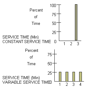
   Thus, we see two different situations can have the same average service times. Simulation is a technique which can be used to mimic (model) real situations which include uncertainties. The simulation itself is a procedure which behaves like the real process.

   We begin by selecting the number of arrivals at time = 0 according to this frequency data.

   

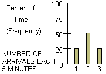
   In this example we shall assume that all of the customers for a given five minute interval arrive at the beginning of the interval.

   Now, how can we choose a number of arrivals? Clearly we want a way which is twice as likely to choose 2 arrivals as either 1 or 3. One way to simulate the number of arrivals at the beginning of a five-minute interval would be to choose at random an integer from 0 to 99. The phrase "at random" means every integer has an equal chance of being selected. We could simulate one arrival, if any integer 0 to 24 was chose, two arrivals if any integer 25 to 74 was chosen, and three arrivals if any of the 25 integers 75 to 99 was chooses. Clearly, this approach does fulfill our need to select two arrivals twice as frequently as either 1 or 3.

3. What number of arrivals would correspond to each of the following random numbers:
   • 16?
   • 25?
   • 96?
   • 47?

4. In fact, if the numbers are drawn at random, what percent of the time will:
   • 1 arrival every 5 min occur?
   • 2 arrivals every 5 min occur?
   • 3 arrivals every 5 min occur?

But these are exactly the frequencies at which our data told us that our arrivals should occur. Thus, to find the numbers of arrivals at t = 0 and t = 5, for example, all we need to do it (1) obtain 2 random integers from 0 to 99; (2) find the corresponding number of arrivals, and (3) mark them on the "arrival" line of our chart at the appropriate times. The process should be continued to find the number of arrivals occurring at the beginning of succeeding five minute intervals. It can also be noted that c1 begins service at t = 0. But how long is c1's service time?

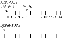
We now apply the same concept to determine service times for each of our five customers. The original service time chart appears below.

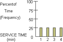
By selecting random numbers from 0 to 99, we can perform the calculations (e.g. average waiting time, time until first no-wait customer, etc). If we repeat the process with new random numbers, the results would be different. Therefore, if we want to get a true evaluation of such a variable rate process, the results of many such calculations should be reviewed and analyzed. For example, the waiting times should be computed for many repeats of the situation and reviewed to see the average, maximum, and minimum values that it takes on.